Das Integral über einem Intervall \([a,b]\) lässt sich an einer Zwischenstelle \(a\le c \le b\) aufspalten. Das Integral über das gesamte Intervall \([a,b]\) ist dann die Summe der Integrale über die einzelnen Intervalle \([a,c]\) und \([c,b]\).

Die folgende Animation zeigt eine Kurve, deren Integral im Intervall \([-2,1.5]\) den Wert \(2.81\) annimmt. Das Intervall wird durch \(c\) in zwei Intervalle unterteilt. Das Integral im Intervall \([-2,c]\) ist blau eingefärbt. Das Integral im Intervall \([c,1.5]\) ist rot eingefärbt. Der Schieberegler kann zwischen \(-2\) und \(1.5\) beliebig in \(0.1\)-Schritten bewegt werden.

Wie zu erwarten ist, verringern Bereiche unterhalb der \(x\)-Achse den Wert des Integrals.

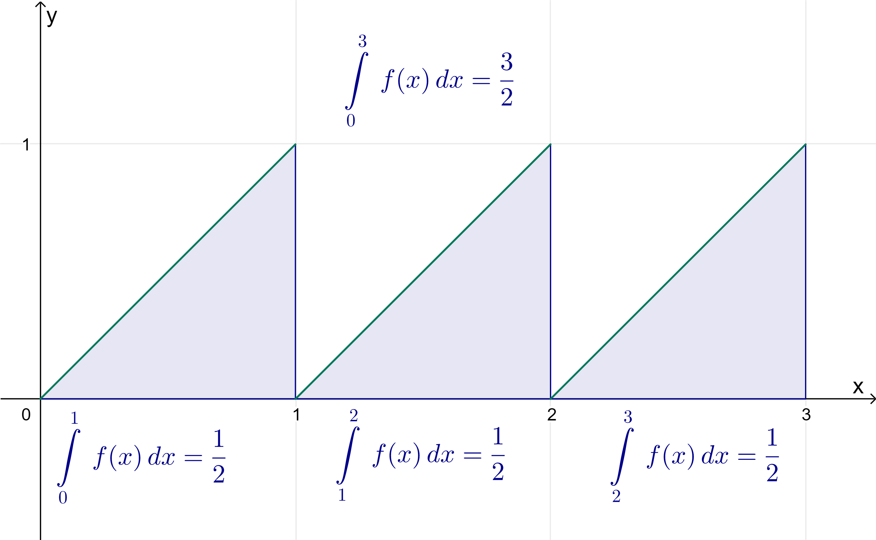
Wir betrachten die Funktion \(f:[0,3]\longrightarrow\mathbb{R}\) mit

\(\qquad f(x)=\left\{\begin {array} {}x & \textsf{für} & 0\le x\lt 1 \\ x-1 & \textsf{für} & 1\le x\lt 2 \\ x-2 & \textsf{für} & 2\le x\le 3  \end {array} \right.\)

und berechnen \(\displaystyle\int \limits _0^3 f(x)\, dx\):

\(\qquad \displaystyle\int \limits _0^3 f(x) \, dx = \displaystyle\int \limits _0^1 x \, dx+ \displaystyle\int \limits _1^2 x-1 \, dx+ \displaystyle\int \limits _2^3 x-2 \, dx\)

\(\qquad \phantom{\int \limits _0^3 f(x) \, dx} = \left[\dfrac{x^2}{2}\right]_0^1+ \left[\dfrac{x^2}{2}-x\right]_1^2 + \left[\dfrac{x^2}{2}-2x\right]_2^3\)

\(\qquad \phantom{\int \limits _0^3 f(x) \, dx} =\dfrac{1}{2} + \underbrace{\left(\dfrac{2^2}{2}-2\right)- \left(\dfrac{1^2}{2}-1\right) }_{\dfrac{1}{2}}+\underbrace{ \left(\dfrac{3^2}{2}-2\cdot 3\right)-\left (\dfrac{2^2}{2}-2\cdot 2\right)}_{\dfrac{1}{2}}\)

\(\qquad \phantom{\int \limits _0^3 f(x) \, dx} =\dfrac{1}{2} +  \dfrac{1}{2}+ \dfrac{1}{2}=\dfrac{3}{2}\)